DCF Terminal Value Methods

Ask any analyst who has ever created their first time DCF why terminal value is important, and he or she will tend to answer you in a technically correct but incomplete manner. They will claim it reflects the value outside the explicit period of the forecast. What they fail to recognize is that a large part of the total enterprise value that a single number reflects, in most instances, 60 to 80 percent of the valuation product. That causes the terminal value calculation DCF not to be simply a bottom-line item on a model, but perhaps the most significant group of assumptions in the whole analysis.

In the case of junior to mid-level finance people, creating a discipline-based grasp of terminal value, and its calculation, where it might go awry, and how it can be stressed, is one of the quickest methods to increase the quality of their analysis. The terminal value section of your model will certainly face the most scrutiny by senior reviewers and clients alike, whether you are preparing a valuation to support an M&A transaction, supporting a fundraising process, or conducting a startup valuation using DCF.

The two main approaches to estimating terminal value, the Gordon Growth Model and the Exit Multiple Method, are clearly and practically explained in this article, and how they are combined into a complete DCF framework. It also discusses the special problems that can occur in using discounted cash flow valuation techniques with high-growth or pre-profit companies, and concludes with 5 principles that ought to inform the practice of every practitioner. Throughout, it uses real-life scenarios and sensitivity examples to make the concepts a reality.

The Role of Terminal Value in a Complete DCF

The DCF model is constructed in two components. The former is the explicit forecast period – generally, five to ten years of projected free cash flows, constructed line by line based on revenue assumptions down to operating costs, taxes, changes in working capital, and capital expenditure. The latter is all the rest: the final value. Combining the two elements, the present value amounts to the enterprise value of the business in question.

Terminal value is given this degree of attention not because it is conceptually deserving, but more due to mathematical reasons. A very small business with a growth rate of 2 per cent forever after Year 5 will increase in value to a terminal value far larger than the value of its explicit forecast cash flows, merely because that perpetual stream of cash, when discounted, will grow over an infinite horizon. It is not a modeling gimmick, but is a consequence of the economic reality that a going concern is more valuable than can be predicted within any finite time horizon. This is the key to all discounted cash flow valuation techniques, whether it is a stable utility or an exponentially growing technology company.

The inherent problem with terminal value is, however, that it is more assumption-based than the explicit period is. During the first five years, a manager can refer to management advice, past growth rates, contracted revenues, or competitor standards to back up every line. The assumptions are more hypothetical beyond the forecast horizon. This is the reason why the two primary methods, the Gordon Growth Model and the Exit Multiple Method, are nearly always applied in cross-check and not single.

Gordon Growth Model vs. Exit Multiple Method

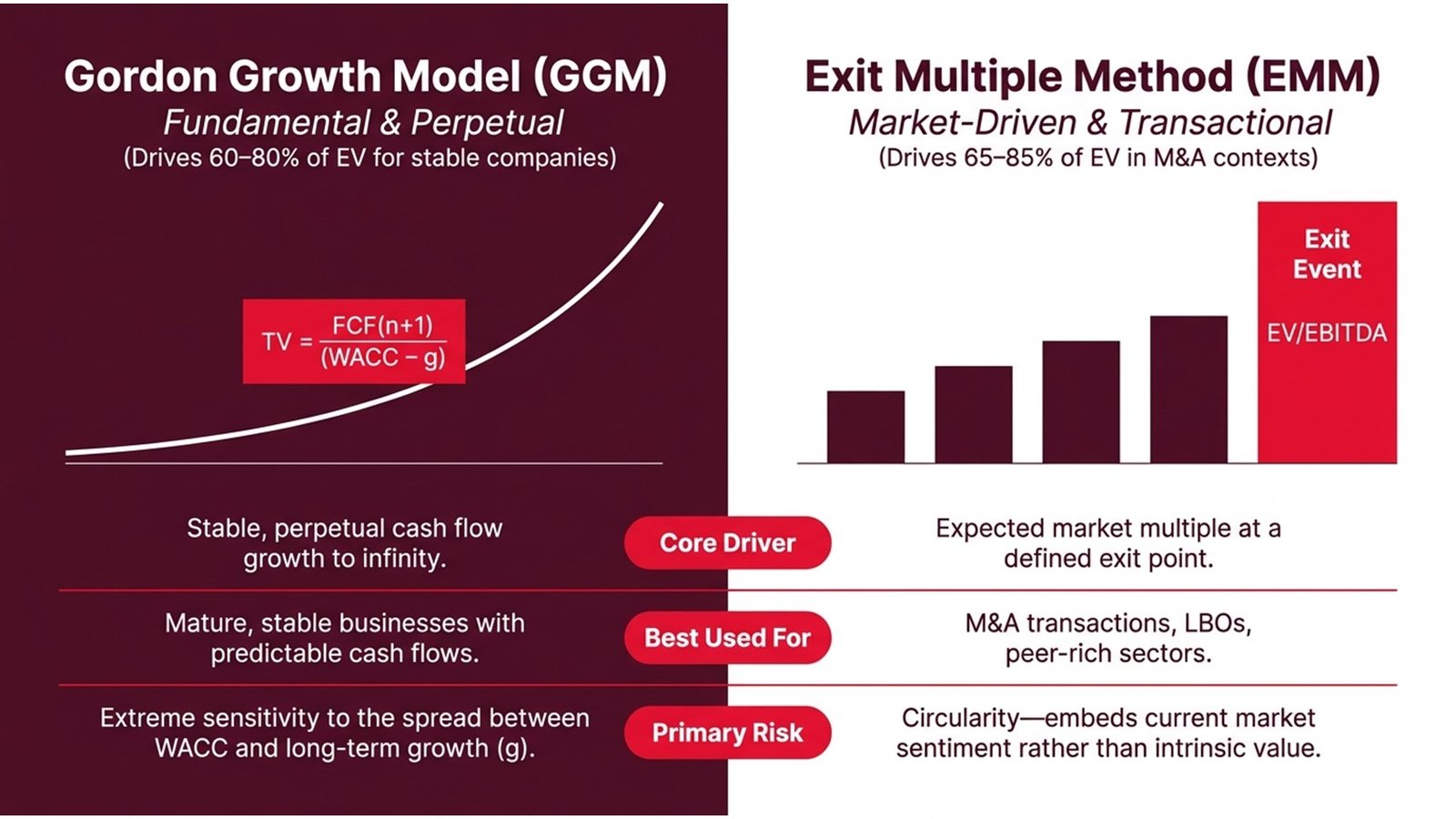
The Gordon Growth Model (sometimes known as the perpetuity growth model) obtains the terminal value by dividing the normalized free cash flow in the final year by the difference between the discount rate (WACC) and the estimated long-term growth rate. This is simple, TV = FCF(n+1)/(WACC -g). The figure obtained is then discounted to the present. The beauty of this method is that it is very simple; the risk is that the output is highly sensitive to the difference between WACC and g. A one-percentage-point change in either variable may alter the terminal value – and thus the overall enterprise value – by 20 to 30 percent or more.

The Exit Multiple Method looks at the terminal value as a market approach as opposed to a fundamental approach. Rather than extending cash flows to infinity, the analyst, based on the explicit forecast period, makes a series of assumptions that the business sells at the end of the explicit forecast period at a multiple of EBITDA, EBIT, or revenue that is reflective of what similar companies are trading at present. The multiple is then replicated on the projected metric at the end of the year, and the end value is the produced terminal value that portrays the current market conditions. The attractiveness of the approach is that it is intuitively associated with the transaction markets – it is a reflection of the pricing of the real deals. Its weakness is that it may be circular: when similar company multiples are also calculated using DCF valuations, to base the value of your own DCF on them is to add a layer of dependency on market sentiment that may be hard to disaggregate.

Each technique has its valid uses, and the most skilled analysts employ both. The gap itself is analytically useful when there is a material difference between the terminal value determined by the two methods, e.g., the GGM suggests an enterprise value of 500 million, and the Exit Multiple Method suggests an enterprise value of 700 million. The question arises: is the market today over-priced on fundamental value in this sector, or is my long-term growth assumption too conservative? Good terminal value calculation DCF work is all about that type of interrogation.

Table 1: Gordon Growth Model vs. Exit Multiple Method — A Practical Comparison

Criterion	Gordon Growth Model (GGM)	Exit Multiple Method (EMM)
Core Assumption	The cash flows increase at a constant, indefinite rate.	Business is sold at a multiple of exit, which is derived from the market.
Key Inputs	Final year FCF, WACC, long-term growth rate(g).	Final year EBITDA (or EBIT/Revenue) and chosen multiple
Best Used For	Well-established and stable businesses with stable cash flows.	M&As, LBOs, similar company-rich industries.
Main Risk	Very delicate to the diffusion between WACC and g.	Captures the present-day mood of the market – may be circular.
Typical TV / Total Value	60–80% of enterprise value for stable companies	65–85% of enterprise value in M&A contexts

Five Principles for Building a Defensible Terminal Value

To construct a terminal value that can withstand scrutiny, whether by a client, a senior partner, or an investment committee, a formula may be needed, but it is not sufficient to simply enter some numbers into the formula. The five principles that follow are lessons learnt painfully by practitioners who have worked in the various fields of investment banking, in the private equity, as well as the corporate development, and they apply regardless of which method you are applying, either the GGM, the Exit Multiple Method, or both.

1. Always cross-check both methods

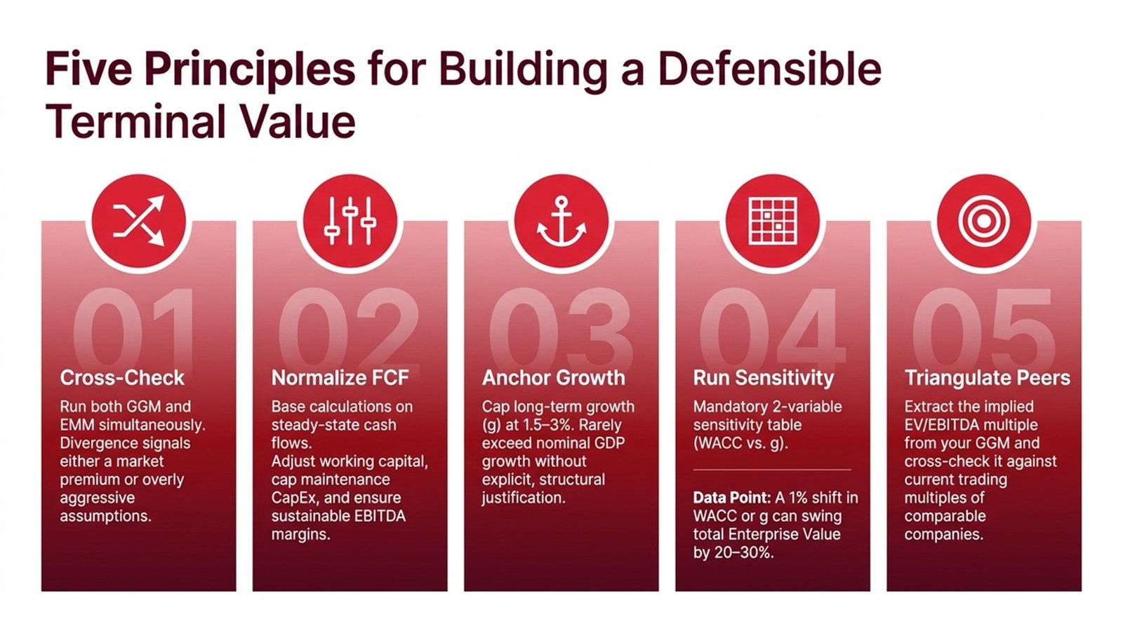
It is a professional risk to be dependent on a single approach. Take the Gordon Growth Model as your main line of analysis and the Exit Multiple Method as your market-reality test. When the implied exit multiplier of your GGM-calculated terminal value makes no sense in comparison with levels in similar companies in the market today, there is something that needs to be amended in your assumptions. This cross-check is the norm in investment banking and in private equity environments, and the absence of it is an indication of a lapse in analytical rigor.

2. Normalize the terminal year FCF carefully

The amount of cash flow that you will use to seed the GGM must reflect a normal, steady-state amount of earnings, not the actual production you will produce at the end of your projection year. The adjustments generally involve normalizing changes in the working capital, making sure that CapEx shows maintenance-level expenditure instead of a growth spurt, and establishing that the EBITDA margin of the last year is in line with industry standards of a mature company of this kind. One of the most frequent mistakes identified in junior analyst work is the failure to normalize, and it can lead to the terminal value being materially overstated or understated.

3. Keep the long-term growth rate anchored in reality

Growth rate over a long period exceeding what is expected of the growth of the nominal GDP rate of the economy is hardly justifiable in a mature business. This is logical because no company can develop higher than the economy in the long run without becoming the whole economy. In the case of most developed market businesses that are stable, a long-term growth rate of 1.5 to 3 percent is acceptable. In the case of a business with structural tailwinds, such as healthcare services, some segments of technology infrastructure, the upper limit of that range, or a tad higher, can be justified, but must be explicitly so.

4. Run a formal sensitivity analysis

Since the terminal value is such a sensitive matter to the WACC-minus-g spread, it would be no more than a minimum requirement to construct a two-variable sensitivity table of the enterprise value in a system of discount rates and growth rates. The following table shows the extent of changes in terminal value even under a small set of assumptions. The key to all serious discounted cash flow valuation techniques is to understand these dynamics.

Table 2: Terminal Value Sensitivity — Illustrative GGM Output ($M) | Final Year FCF = $10M

WACC \ Growth Rate (g)	1.5%	2.0%	2.5%	3.0%
8%	$142M	$167M	$200M	$250M
9%	$118M	$133M	$154M	$182M
10%	$100M	$111M	$125M	$143M
11%	$86M	$94M	$104M	$118M

5. Triangulate with a comparable company check

When you have computed your terminal value using both approaches, take out the implied EV/EBITDA multiple of both and find the difference with the trading multiples of your peer group. When the value of the terminal value that you have calculated using GGM suggests a 14x EBITDA multiple and similar companies are trading at 8-10x, you either have a real premium that the market ought to be paying to this business, or you have overestimated your growth assumptions. Triangulation exercise maintains the analysis in market reality, and this is particularly crucial when the model is going to be applied in a negotiation or a presentation at the board level.

Process Flow 1: Full DCF Workflow — From Revenue Forecast to Enterprise Value

Step 1	Step 2	Step 3	Step 4	Step 5	Step 6
Forecast Explicit Period	Estimate WACC	Project Terminal Year FCF	Calculate Terminal Value	Discount All Cash Flows	Derive Enterprise Value
Build a 5–10 year free cash flow forecast from revenue to unlevered FCF	Weighted cost of equity (CAPM) and after-tax cost of debt by capital structure	Normalize FCF of working capital, CapM, and sustainable margin.	Use GGM or Exit Multiple; compare with the other technique.	Revive explicit FCFs and TV with WACC.	Sum PV of FCFs + PV of TV; add cash, subtract debt for equity value

Applying These Methods to Real Scenarios

Theoretical knowledge of terminal value is one thing; it goes another to put it into practice when faced with a real deal or valuation assignment. Three scenarios help us understand the ways and principles of the above-discussed methods and principles in practice, and each scenario has a different lesson.

Take the example of a mid-market industrial manufacturer in Germany first – a family-owned company with constant EBITDA margins of about 14 percent, with revenue increasing at an annual rate of about 4 percent. The primary method, which is natural in this case, is the Gordon Growth Model. The growth rate in the long term is determined at 2 percent (generally consistent with the Eurozone nominal GDP growth), and the difference between WACC and g yields a terminal value that approximates 65 percent of the total enterprise value. The Exit Multiple Method, with a 7x EBITDA multiple (in line with similar European industries deals), generates a figure that is within 8 percent of the GGM data – a comfortable area of convergence that provides the analyst with confidence in the output. This type of cross-check is a commonplace anticipation in European M&A advisory practice where purchasers and their advisors are both savvy and assumptions are under the microscope.

The second case is about a direct-to-consumer healthcare brand that is in the United States with a high growth rate of 80 million in revenue and 4 million in EBITDA as it pushes to acquire more customers. In this case, the GGM of current-year FCF would give an insignificant value – the normalized FCF is too low to represent the inherent value of the business. Rather, the analyst goes further and projects the explicit forecast to Year 8, upon which the model predicts that the EBITDA margins would have stabilized at 18 percent. That normalized Year 8 FCF is then used to anchor the terminal value and cross-referenced with an exit multiple of 12x EBITDA that is also in line with other similarly-based specialty health and wellness firms. This situation exemplifies one important rule: the duration of the explicit forecast period must be dictated by the time at which the business is in a truly steady state rather than custom. This is more so in the context of startup valuation using DCF, where steady-state profitability can be half a decade or more distant.

Terminal Value Challenges in Startup and High-Growth Contexts

The terminal value challenges are further enhanced when the start-up valuation is based on DCF when dealing with pre-profit, fast-growing, or in an industry with little to no well-established comparable set. Such cases are becoming increasingly frequent as VVC-backed companies seek subsequent capital investments and strategic acquirers consider acquisition targets with high growth potential. The common DCF model must be substantially modified to be believable in such situations.

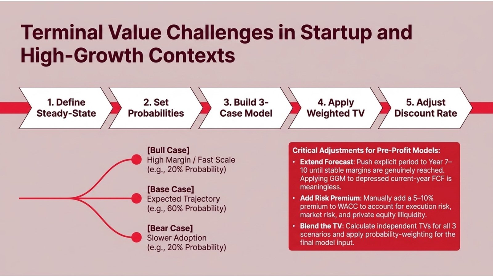
The most feasible adjustment is the application of the scenario-weighted terminal values. Instead of basing on a single base-case FCF, the analyst constructs three independent cases, bear, base, and bull, and each has its own revenue path, margin path, and terminal year assumptions. Each scenario is allocated a probability depending on evidence in the market, the dynamics of competition, and the management track record. Each scenario is then calculated separately, and then the weighted average results are the blended terminal value input into the DCF. This method is more justifiable than a one-case model since it will expose the risk, as opposed to hiding it in a single growth rate assumption.

Another dilemma connected to the startup situations is the selection of the discount rate. The use of standard WACC, based on the observed beta of similar publicly traded businesses, frequently underestimates the actual risk of an early-stage business. To estimate the execution risk, market risk, and the illiquidity risk of the equity of a private company, many practitioners would take a particular risk premium of 5 to 10 percentage points on top of the calculated WACC. This modification has a material impact on the terminal value, which is the right thing to do, as it is the real uncertainty. The inability to do this repricing is among the methods through which the discounted cash flow valuation methods can generate bloated and ultimately inaccurate valuations of start-up businesses.

Process Flow 2: Adapting the DCF for Startup and High-Growth Businesses

Phase 1	Phase 2	Phase 3	Phase 4	Phase 5
Define Steady-State Year	Set Scenario Probabilities	Build Three-Case FCF Model	Apply Probability-Weighted TV	Adjust Discount Rate
Determine when the startup is stable with respect to margins (usually Year 7-10)	Weight base, bull, and bear cases according to market evidence.	Forecast revenue → EBITDA → FCF under each scenario independently	TV for each scenario, probability blended TV.	WACC should be increased by a risk premium (5-10) to indicate uncertainty at the early stages.

Conclusion: Building Terminal Value Discipline

The terminal value is such that a DCF model is either gaining or losing its credibility. Since it is such a high proportion of the overall enterprise value, any error or unwarranted assumption in this section disproportionately affects the ultimate output, much more than an equivalent error in the Year 3 forecast of revenues. Learning how to make real discipline in terminal value calculation, DCF is thus amongst the most significant investments that any finance professional can make in their technical abilities.

A number of tangible steps are based on all the contents of this article. To start with, always include in your DCF the Gordon Growth Model and the Exit Multiple Method, and record the implied multiples of each. Second, scale your terminal year FCF to the normal before entering it into the GGM – this is the only thing you can do to get rid of one of the most typical errors in the work of junior analysts. Third, maintain your long-run growth rate in the realm of economic fundamentals, and only when you are tempted to exceed 3 percent, be able to justify the assumption by sector-specific facts, not by wishful thinking.

Fourth, never just take a point estimate of WACC and g, but always do a sensitivity analysis on these two variables and report the result as a table with two variables. It is not only good modeling practice, but a tool in communication that assists decision-makers to see the spectrum of results as opposed to basing decisions on one number. Fifth, to startup valuation using DCF, extrapolate your explicit forecast to a true steady state of the business, apply scenario-dependent terminal values, and apply a suitable risk premium to your discount rate.

Lastly, it is important to remember that a terminal value is a model output and not a fact. Its most effective practitioners consider it a structured hypothesis – one that is internally coherent, market-sensitive, and requires specifying its assumptions. Whenever reviewers, clients, or investment committee members are asking questions about your terminal value, they are not seeking certainty; they are seeking rigour and judgment. It is these two characteristics, rather than any formula or shortcut, that make the difference between good and discounted cash flow valuation techniques and shallowly polished work that does not stand the test of time.